How Expected Goals (xG) Can Improve Football Match Analysis?

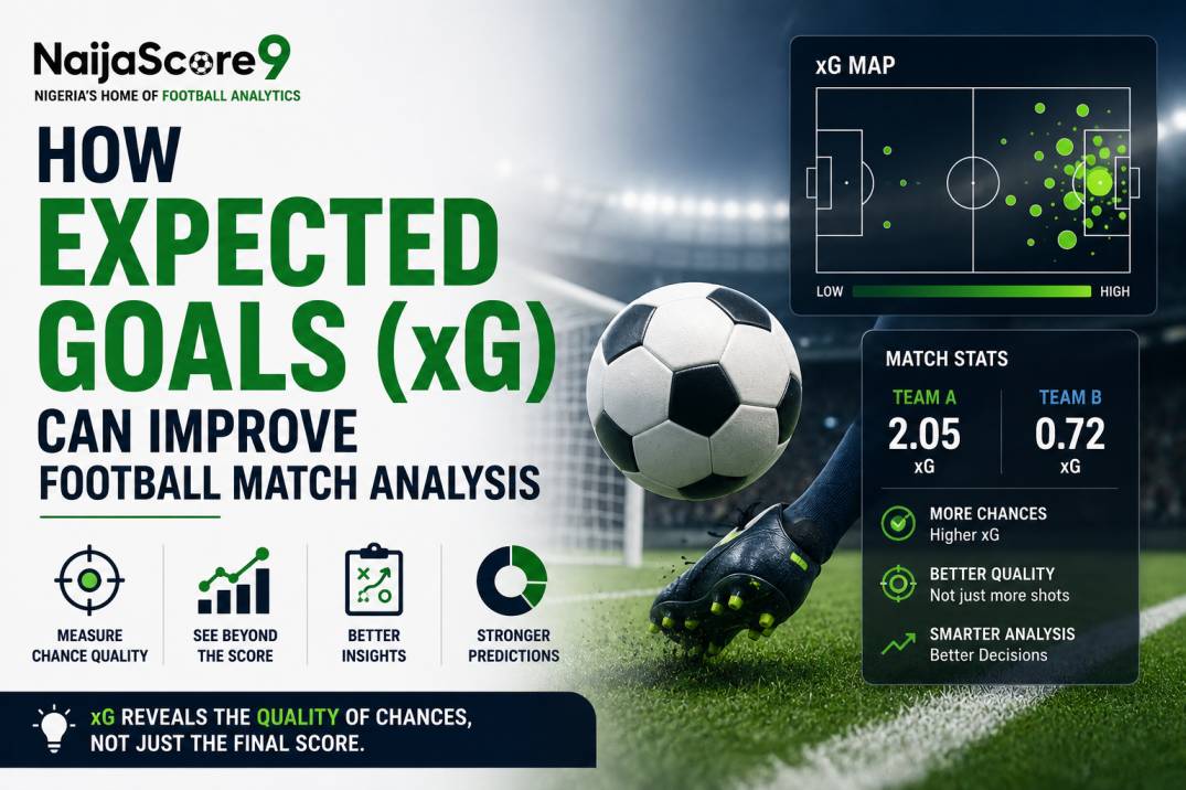
A team wins 2–0 and appears to have produced a comfortable performance.

Then you look at the underlying chances:

Team A: 0.72 xG
Team B: 2.05 xG

The score says Team A won convincingly. The chance quality tells a different story: Team B created the better opportunities but failed to convert them.

That is where expected goals (xG) becomes useful.

Traditional results tell you what happened. xG helps explain how those goals, or missed goals, were created.

For football match analysis, this distinction matters because a recent run of wins can hide weak performances, while a run of defeats can sometimes hide a team that is consistently creating good chances and conceding relatively little.

Used properly, xG can improve football predictions by helping you evaluate:

• the quality of chances a team creates;
• the quality of chances it concedes;
• whether recent results are supported by underlying performances;
• whether finishing or goalkeeping has been unusually strong or weak;
• how two teams’ attacking and defensive profiles match up.

But xG is not a score predictor by itself.

A strong analysis uses it alongside team news, tactical match-ups, home and away performance, expected line-ups, fixture congestion and other relevant information.

What Is Expected Goals (xG)?

Expected goals measures the probability that a shot will become a goal based on the characteristics of that chance.

An xG value normally runs from:

0 to 1

A shot rated:

0.10 xG

represents roughly a 10% scoring chance according to that particular model.

A chance rated:

0.60 xG

is considered substantially more likely to result in a goal.

StatsBomb describes xG as a probability assigned to a shot using historical information from similar chances. Common model inputs include factors such as distance from goal, shooting angle, body part and the action that created the shot. Opta uses the same underlying principle: evaluating how likely a chance is to be scored by comparing it with large numbers of historical shots.

This means xG does something that a basic shot count cannot.

Consider:

Team A: 15 shots
Team B: 7 shots

At first glance, Team A appears far more dangerous.

But suppose:

Team A: 15 shots, 0.75 xG
Team B: 7 shots, 1.90 xG

Team A took more shots, but Team B generated fewer and much better opportunities.

That is why xG can improve match analysis.

How Is a Team’s Match xG Calculated?

A team’s total xG is broadly the sum of the xG values assigned to its shots.

For example:

Chance	xG
Shot 1	0.08
Shot 2	0.14
Shot 3	0.37
Shot 4	0.09
Shot 5	0.52
Total xG	1.20

The team created approximately 1.20 xG from those chances.

That does not mean the team “should definitely have scored 1.2 goals.”

You cannot score 0.2 of a goal.

It is an estimate of the combined quality of the team’s shooting opportunities.

Over one match, the actual result can differ sharply from xG.

Over a larger sample, the metric becomes more useful for understanding underlying attacking and defensive performance.

Why the Final Score Can Be Misleading?

Football is a low-scoring sport.

A small number of events can have a large effect on the final result:

• an excellent finish;
• a goalkeeper error;
• a penalty;
• a deflection;
• a shot hitting the post;
• a missed one-on-one.

Consider two matches.

Match A

Team X wins:

3–0

xG:

Team X 1.05 – 1.20 Team Y

Match B

Team Z draws:

0–0

xG:

Team Z 2.15 – 0.42 Team W

Looking only at results, Team X appears impressive while Team Z appears ineffective.

Looking at chance creation, the interpretation changes.

Team X scored three times from a relatively modest collection of chances while allowing the opponent comparable opportunity.

Team Z dominated the quality of chances but failed to convert.

For the next fixture, that underlying information can be more useful than treating 3–0 as automatically “good form” and 0–0 as automatically “poor attack.”

Opta specifically notes that xG is useful for evaluating underlying performance because teams and players can score above or below the quality of chances they generate.

The Four xG Numbers That Matter Most

For practical match analysis, you do not need dozens of advanced statistics.

Start with four.

1. xG For

xG For (xGF) measures the quality of chances a team creates.

If a team regularly produces:

1.8–2.0 xG per match

it is generating stronger attacking opportunities than a team regularly around:

0.7–0.9 xG

But the number should be interpreted relative to:

• opposition quality;
• venue;
• league;
• match state.

2. xG Against

xG Against (xGA) measures the quality of chances a team allows opponents to create.

A team conceding only:

0.80 xGA per match

may have a more sustainable defensive profile than one conceding:

1.70 xGA

even when both have conceded the same number of actual goals recently.

3. xG Difference

A simple xG difference is:

xGF − xGA

Suppose:

Team A:

1.75 xGF − 0.90 xGA = +0.85 xG difference

Team B:

1.15 xGF − 1.55 xGA = −0.40 xG difference

Team A is not merely creating more chances. It is also allowing fewer high-quality chances.

That balance can be more informative than looking only at goals scored.

4. Non-Penalty xG

Penalties are high-quality opportunities and can heavily influence a small xG sample.

If a team produces:

2.1 xG

but:

0.8 xG

comes from one penalty, its open-play attacking performance was closer to:

1.3 non-penalty xG

That is still useful, but it tells a different story.

When evaluating repeatable attacking quality, separating penalties can prevent one isolated event from dominating the analysis.

How xG Can Improve Football Predictions?

The main value of xG in prediction work is not that it gives you an automatic winner.

Its value is that it helps correct some of the weaknesses in result-based analysis.

1. xG Can Expose Unsustainable Winning Form

Suppose a team has won five consecutive matches.

Results:

2–0
1–0
3–1
2–1
1–0

That looks like excellent form.

Now examine the cumulative numbers:

Goals scored: 9
Goals conceded: 2

But:

xG created: 5.2
xG conceded: 7.0

The team has scored considerably more than the quality of its chances and conceded considerably fewer goals than the opportunities allowed.

That does not guarantee the winning run will end.

It does suggest that:

The results have been stronger than the underlying performances.

For the next match, blindly using “five straight wins” may therefore overstate the team’s current strength.

2. xG Can Identify Better Performances Hidden by Poor Results

Now consider the opposite case.

A team has:

1 win, 1 draw, 3 losses

in its last five.

Goals:

4 scored
7 conceded

But its underlying numbers are:

7.1 xG created
4.8 xG conceded

The results look weak.

The chance creation looks much stronger.

Possible explanations include:

• poor finishing;
• strong opposing goalkeeping;
• defensive errors on a small number of chances;
• short-term variance.

This does not automatically make the team a strong prediction for its next game.

But it tells you to investigate further rather than simply labelling the team “out of form.”

This is one reason xG football analysis is often more useful than reading a form table alone.

3. xG Helps Separate Shot Quantity From Shot Quality

Imagine two teams.

Team A

Average shots:

16

Average xG:

1.25

Team B

Average shots:

10

Average xG:

1.70

Team A takes six more shots per match.

But Team B creates higher-quality overall shooting opportunities.

This can happen because Team A repeatedly shoots from:

• long range;
• difficult angles;
• crowded positions.

Team B might generate fewer attempts but create more:

• cutbacks;
• one-on-ones;
• close-range chances;
• central penalty-area shots.

For predicting future goals, the quality of the opportunities matters.

A large shot count by itself can exaggerate the attacking threat.

4. xG Can Improve Defensive Analysis

Most xG discussion focuses on attacking teams.

But xG against can be just as valuable.

Suppose two teams have conceded six goals across their last six matches.

That appears equal.

But:

Team A

6 goals conceded from 4.1 xGA

Team B

6 goals conceded from 10.0 xGA

Team A has allowed relatively limited chance quality but conceded slightly more than expected.

Team B has been giving opponents enough opportunities to score far more often.

Their defensive records look identical in the goals column.

Their defensive processes do not.

When analysing the next opponent, Team B’s defence deserves much greater concern.

5. xG Can Help Evaluate Over/Under Goals

Expected goals can also provide context for total-goals markets.

Suppose Team A averages:

1.85 xGF
1.45 xGA

and Team B averages:

1.60 xGF
1.55 xGA

Both teams regularly participate in matches with substantial chance creation.

That can support a higher expected scoring environment.

But do not simply calculate:

1.85 + 1.60 = expected match goals

That would ignore how each attack interacts with the opposing defence.

A stronger approach considers:

Team A attack vs Team B defence

and:

Team B attack vs Team A defence

Then adjust for:

• venue;
• expected line-ups;
• tactical style;
• injuries;
• match importance;
• pace of play.

xG should strengthen the analysis—not replace it with one arithmetic shortcut.

6. xG Can Improve BTTS Analysis

For Both Teams to Score, the useful question is not merely:

Have both teams scored frequently recently?

Consider:

Team A

Scored in 8 of last 10.

But averages:

0.95 xG per game

Team B

Scored in only 6 of last 10.

But averages:

1.65 xG per game

The historical scoring frequency favours Team A.

The underlying chance creation favours Team B.

For a future BTTS assessment, xG can help determine whether recent scoring records are supported by the chances being generated.

The same principle applies defensively.

A team that has kept three recent clean sheets while conceding:

1.8, 2.0 and 1.6 xGA

has probably been much more vulnerable than the clean-sheet record suggests.

7. xG Can Strengthen 1X2 Match Analysis

A home-win prediction should not come from xG alone.

But xG can help compare the teams’ underlying strength.

Consider:

Metric	Home Team	Away Team
xG For	1.82	1.15
xG Against	0.94	1.56
xG Difference	+0.88	-0.41
Home/Away context	Strong at home	Weak away

The home side has:

• stronger chance creation;
• lower-quality chances conceded;
• a much healthier overall xG difference.

That supports the case for the home side.

But before turning it into a probability, you still need to check:

• missing players;
• expected formation;
• rest;
• fixture congestion;
• opponent strength;
• market price.

NaijaScore9’s football prediction methodology uses this broader principle: no single metric should be treated as conclusive, and match probabilities need to be interpreted together with current context. NaijaScore9 prediction pages already combine probability splits and expected-goal information with other match signals rather than presenting xG as a standalone answer.

Use Recent xG Carefully

Recent xG is useful.

But a five-match sample can still mislead.

Suppose a team’s last five xG figures are:

2.10
1.95
2.30
2.05
1.80

That appears very strong.

Now check the opponents.

All five were among the league’s weakest defensive teams.

The next opponent has the best defensive record in the competition.

Simply carrying the 2.04 average into the next match can substantially overestimate the attack.

Recent xG should therefore be adjusted for:

who the team played.

The same applies to xGA.

A defence that looks excellent after facing three weak attacks may be less impressive than the raw figures suggest.

Home and Away xG Should Be Separated

Football teams can perform very differently depending on the venue.

Suppose a club averages:

Overall xGF: 1.50

That number looks reasonable.

But split it:

Home xGF: 2.05
Away xGF: 0.95

For an away prediction, the overall 1.50 figure is not the most relevant number.

The same applies to defensive performance:

Home xGA: 0.90
Away xGA: 1.55

If the next match is away, the weaker away profile deserves more weight.

For practical xG football predictions, use the context closest to the upcoming fixture rather than relying only on a season-wide average.

Game State Can Distort xG

One of the most important xG limitations is game state.

Suppose Team A goes 2–0 ahead after 25 minutes.

It may then:

• defend deeper;
• reduce attacking risk;
• concede possession;
• allow the opponent more shots.

The final xG might be:

Team A 1.40 – 1.75 Team B

Looking only at the final xG could make Team B appear superior.

But much of Team B’s chance production may have come while chasing a two-goal deficit against a side protecting its lead.

Now reverse the situation.

A team trailing 1–0 for 70 minutes may generate a large amount of late xG because it pushes players forward.

That does not necessarily mean it controlled the match from the beginning.

When analysing xG, ask:

When were the chances created, and what was the score at the time?

The final total is useful.

The match story still matters.

Red Cards Can Make xG Comparisons Misleading

Suppose a team records:

2.4 xG

against an opponent that played with ten men from minute 25.

That attacking performance should not be interpreted like 2.4 xG created against eleven players for 90 minutes.

Red cards can change:

• territory;
• shot volume;
• defensive shape;
• possession;
• transition frequency.

If a recent match contains an early sending-off, separate it mentally from normal 11-v-11 performance.

Otherwise, one unusual game can distort a short recent-xG average.

Penalties Can Inflate a Single Match

Penalties are legitimate scoring chances.

They should not simply be deleted from analysis.

But they should be recognised separately.

Suppose Team A produces:

1.95 xG

including:

two penalties

Its open-play chance creation may actually have been modest.

If your next-match prediction assumes the team repeatedly generated 1.95 xG from normal attacking play, you may overestimate its attack.

This is why non-penalty xG (npxG) can be useful when assessing the sustainability of team performance.

Do Not Treat xG Overperformance as Automatic Regression

Suppose a striker has:

10 goals from 6.8 xG

It is tempting to say:

“He must regress because his goals are higher than his xG.”

That is too simplistic.

Some players can finish above average for meaningful periods, and individual finishing ability can matter.

Likewise, goalkeeper quality can influence goals conceded relative to pre-shot xG.

The correct interpretation is:

The player has scored more than the average expectation assigned to those chances. Investigate whether the difference is likely to persist.

Do not automatically subtract future goals simply because historical goals exceeded xG.

Different xG Providers Can Show Different Numbers

You may see the same match listed as:

1.62 xG

on one platform and:

1.84 xG

on another.

That does not necessarily mean one is wrong.

xG models can use different:

• historical datasets;
• shot classifications;
• contextual variables;
• goalkeeper information;
• defensive-positioning information.

StatsBomb explicitly notes that xG models have their own characteristics and can assign different values to the same chance.

For analysis, consistency matters.

If you are comparing a team’s last ten matches, use the same xG provider where possible rather than mixing values from several different models.

xG Is More Useful Over a Sample Than One Match

One match contains substantial randomness.

Suppose a team produces only:

0.55 xG

in one game.

That alone does not prove the attack is poor.

Maybe:

• it faced the strongest defence in the league;
• its striker was injured;
• it received an early red card;
• it protected a lead.

Now suppose its last ten matches show:

0.72 average xG

under largely normal conditions.

That is much stronger evidence of an attacking problem.

For predictive work, xG becomes more useful when repeated performance is evaluated across a reasonable sample and then adjusted for current circumstances.

A Practical xG Match Analysis Framework

You do not need a complicated model to use xG intelligently.

Work through the fixture in this order.

Step 1: Measure Each Team’s Chance Creation

Check:

• season xGF;
• recent xGF;
• home/away xGF;
• non-penalty xGF.

Do not simply pick whichever number is highest. Understand why it is high.

Step 2: Measure Chance Prevention

Check:

• season xGA;
• recent xGA;
• home/away xGA.

A strong attack facing an equally strong defence requires a different expectation from the same attack facing a team consistently allowing high-quality chances.

Step 3: Compare xG Difference

Calculate the broader balance:

xGF − xGA

Consistently positive teams are creating more quality than they concede.

Consistently negative teams are doing the opposite.

Step 4: Compare xG With Actual Results

Ask whether the team is:

• scoring far above xG;
• scoring below xG;
• conceding well below xGA;
• conceding above xGA.

Large gaps tell you where results and underlying performance disagree.

They are a reason to investigate, not automatically reverse the prediction.

Step 5: Check the Opposition Behind the Numbers

Was the recent xG produced against:

• top teams;
• weak teams;
• ten men;
• rotated cup sides?

Quality of opposition matters.

Step 6: Add Current Match Information

Then include:

• confirmed or expected line-ups;
• injuries;
• suspensions;
• player minutes;
• tactical match-up;
• rest;
• fixture congestion;
• motivation.

A historical xG profile can become less relevant when the players responsible for creating those chances are unavailable.

Step 7: Turn the Analysis Into Probabilities

Only after the football assessment should you estimate:

• home win;
• draw;
• away win;
• expected total goals;
• relevant secondary markets.

NaijaScore9’s football predictions provide home, draw and away probability views alongside expected-goal and comparison information on applicable fixture pages.

Step 8: Compare Probability With the Available Price

A strong xG case for a team does not automatically mean its odds offer value.

Suppose your complete analysis gives a home team:

55% win probability

Fair odds:

1 ÷ 0.55 = 1.82

If the market price is:

1.65

the team can still be the most likely winner while the available price is shorter than your estimate supports.

This is why xG analysis and price analysis should remain separate.

NaijaScore9’s guide to value bets, price, probability and market margin explains how to make that final comparison.

Worked Example: Using xG Before a Match

Consider a fictional fixture:

Rivers United vs City FC

Rivers United

Last eight home matches:

1.72 xGF
0.88 xGA

Actual goals:

15 scored
6 conceded

City FC

Last eight away matches:

0.94 xGF
1.61 xGA

Actual goals:

9 scored
10 conceded

At first glance, the matchup favours Rivers United.

Why?

Their home profile shows:

• stronger chance creation;
• substantially lower xGA;
• positive xG difference.

City FC’s away numbers show:

• limited attacking quality;
• relatively high-quality chances conceded.

Now add context.

Suppose Rivers United’s main striker and leading creative midfielder are both unavailable.

Their historical home xG was partly produced with those players.

You should lower confidence in simply carrying the 1.72 xGF average forward.

Alternatively, suppose City FC’s poor away xGA came largely from matches against the league’s top three attacks.

Then its defensive profile may not be quite as weak as 1.61 suggests.

This example shows why xG improves analysis but does not finish it.

The statistic identifies the underlying pattern.

The analyst still has to determine how relevant that pattern is to the upcoming match.

xG vs Actual Goals: Which Is More Important?

Both answer different questions.

Actual goals decide matches.

xG describes the quality of the chances behind those results.

If you want to know:

Who won?

Look at goals.

If you want to investigate:

How convincing was the performance?

xG can provide more context.

For future match analysis, the strongest approach considers both.

A team repeatedly producing strong xG and strong goal numbers presents a different profile from a team producing strong goal numbers on weak underlying chances.

What xG Cannot Tell You on Its Own?

Expected goals does not directly tell you:

• who will win the next match;
• what the exact score will be;
• whether a team will convert its next big chance;
• whether a goalkeeper will make an exceptional save;
• whether a player will be sent off;
• whether a manager will change tactics;
• whether an injured attacker will start.

StatsBomb describes expected goals as a cornerstone input in predictive modelling, but it remains a measure of chance quality rather than a complete prediction system.

That distinction is crucial.

A sophisticated statistic can still be misused if it is treated as certainty.

Common xG Mistakes in Football Predictions

Using One Match as Proof

A single high-xG performance may be an outlier.

Look for repeated patterns.

Looking at xG For but Ignoring xG Against

Attacking strength is only half the match.

Comparing Raw xG Without Opponent Context

Two identical xG averages can have been produced against very different schedules.

Ignoring Home and Away Splits

Venue can materially change team performance.

Treating xG as Predicted Goals

A team with 2.0 recent xGF is not automatically predicted to score exactly two goals next time.

Ignoring Penalties

A penalty can significantly inflate one match’s xG total.

Ignoring Red Cards

An early sending-off can completely change shot and chance production.

Assuming Goals Above xG Must Immediately Regress

Finishing quality and sample size need consideration.

Mixing xG Providers Without Realising It

Different models can assign different values to the same shots.

Ignoring Line-Up Changes

Historical xG created by players who are unavailable may be less relevant to the upcoming fixture.

Conclusion

Expected goals is most valuable when the scoreboard is not telling the complete story.

A team can win several matches while repeatedly allowing the better chances. Another can struggle for results while consistently producing strong attacking opportunities. Looking only at wins, losses and goals can make those teams appear very different from how they are actually performing.

xG helps reveal that difference.

For practical match analysis, start with xG For and xG Against, compare the team’s underlying chance balance, separate home and away performance, and investigate large gaps between actual goals and expected goals.

Then add the context that the historical numbers cannot know about the next fixture:

• who is available;
• who is expected to start;
• how the teams match up tactically;
• whether fatigue or rotation matters;
• how strong the previous opponents were;
• whether the market price already reflects the same information.

That final step is what prevents xG from becoming another statistic used mechanically.

A team with stronger xG numbers is not automatically the correct prediction. A team that has overperformed its xG is not automatically about to lose. And a 2.0 xG average does not mean two goals will appear in the next match.

The better use of expected goals is more disciplined:

Use results to see what happened. Use xG to understand the chances behind those results. Use current match context to decide how much of that evidence still applies to the next game.

That is how expected goals can genuinely improve football match analysis—and why it works best as one important input within a broader probability-based prediction process rather than as a prediction on its own.